Neural Network [grade 2]
Neural Network: linear classification
grade 2: single perceptron with linear classification
Subject for grade 2 is to develop a linear classification with single perceptron.
We will commence a classification problem: linearly split within a 2D space.
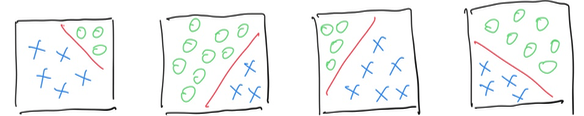
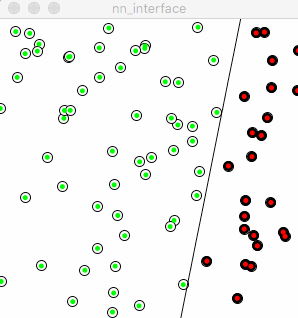
As showed in above picture, green and blue stands for 2 classes, the red lines represent 4 different scenarios in classification.
To solve problem of “linear classification”, 1 perceptron could perform this task.
The network structure remain unchanged with grade 1:

Classification is a typical “supervised learning” in machine learning, which means machine’s performance on predict objects will be measured all the time. When we are saying performance, usually we are talking about the degree of errors.
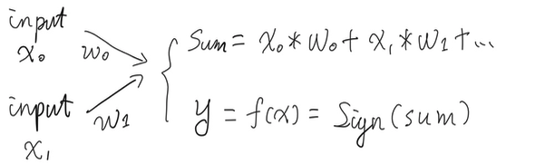
Let’s review data we played with:
- inputs (2 inputs, reason of 2 is which could be easily mapped to the 2D space by transfer them to x and y coordinates);
- weights (initialized by random between 0 to 1);
- outputs (use the sign function to generate -1 and 1);
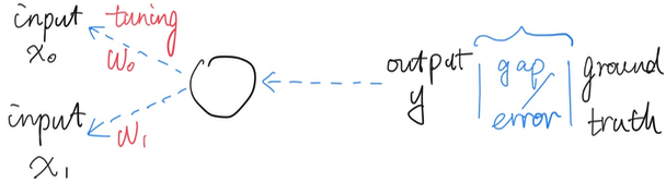
The object here is to accept any of inputs, make the perceptron outputs the rights classification, say “-1” and “1”. Thus the data we could manipulate here is : weights. How do we refine the magic weights, make those help the perceptron doing the right thing?
Just like driving, we wanna make sure that the car is heading the right direction. Here the direction or hint was gave by “error measurement”.
| Actual | Predict | Actual - Predict |
|---|---|---|
| 1 | 1 | 0 |
| 1 | -1 | 2 |
| -1 | -1 | 0 |
| -1 | 1 | -2 |
These are the scenarios on perceptron’s prediction, total in 4. Specifically, line 2 and line 4 are the perceptron making errors, and here we use a simple equation to describe how big is an error:
Error = Actual - Predict
As we discussed, weights are the key to help perceptron does the right thing, here we present the key method in manipulate weights:
Weights += Errors * Inputs * Learning_rate
Learning_rate is one of a hyper-parameters in neural network, which impacts the “speed of learning”, in simple, we could take it as the degree that the current weights will yield to the current errors.
The process of: Compare outputs with actual class, get the degree of errors, passed errors back to input layer, adjust weights accordingly is called: back propagation, or training (tweak outputs according to training data given). By doing this process, the neuron perceptrons are really learning from errors.
Let’s take a look at an simple example: Following is a feed forward process, 2 inputs are 0.5 and 1, 2 randomly assigned weights: 0.1 and -0.5, the perceptron generates output of -1.
| Inputs | Original weights | Sum(inputs * weights) | Sign outputs |
|---|---|---|---|
| 0.5 | 0.1 | 0.5 * 0.1 | |
| 1 | -0.5 | 1 * -0.5 | |
| 0.05 - 0.5 | -1 |
Now assume we are expecting the output of “1” instead of “-1”, let’s see how the back propagation impacts weights:
| Errors | Inputs | Learning_rate | New Weights | Original weights |
|---|---|---|---|---|
| 1 - (-1) | 0.5 | 1 | 2 * 0.5 * 1 | 0.1 |
| 1 - (-1) | 1 | 1 | 2 * 1 * 1 | -0.5 |
Under the original weights combination, 0.1 and -0.5, gave the output of -1. Through back propagation, they were been tweaked into 1 and 2. They were increased especially for the latter: -0.5 was punished, from negative to positive value, aka, the direction of impact was changed.
(Note: “1” is not the usual value for learning rate, we will take a much smaller learning rate in practical. )
Now let’s cook the coding part: On top of predict function in grade 1, we will add another training function within perceptron class in processing:
class Perceptron {
  float[] weights;
  float learning_rate = 0.01;
  float bias = 1.0;

  // Constructor, takes in # of weights and initialize
  Perceptron(int n) {
    weights = new float[n];
    for (int i = 0; i < weights.length; i++) {
      weights[i] = random(1, 2);
    }
  }

  // Generate outputs
  int predict(float[] inputs) {
    float sum = 0;
    for (int i= 0; i < weights.length; i++) {
      sum += inputs[i] * weights[i];
    }
    int predict = sign(sum);
    return predict;
  }

  // Training process
  void train(int label, float[] inputs) {
    int predict_result = predict(inputs);
    int error = label - predict_result;
    if (predict_result == error) {
      return;
    }
    for (int i = 0; i < weights.length; i++) {
      // tune the weight based on previous result and basis
      weights[i] += inputs[i] * error * learning_rate;
    }
  }

  // used to plot classification line
  float guessY(float x) {
    //w0 * x + w1 * y + w2 * bias = 0;
    return -weights[2] * bias / weights[1] -weights[0] * x / weights[1];
  }

  // Activate function, sign is a basic function gets "+" / "-"
  int sign(float sum) {
    if (sum >= 0) {
      return 1;
    } else {
      return -1;
    }
  }

}
A small notice, we used output = input weight + bias weight in the code implementation, with bias = 1 as predefined. [Complete codes on github] https://github.com/hifreedo/nnfs
Following is the animation of how a network with single neuron learns classification, red dot denotes wrong prediction, green means correct prediction, the line in black was drew according to object function, aka y=m*x+b. The line split the 2 categories which are 2 type of nodes on the picture. The red line shows how the network is learning iteration by iteration.
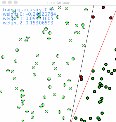
As described in above, the learning rate determines how “fast” or the “scope” of the red line moves. A relatively small learning rate could speed down the learning process, a big learning rate could speed up the learning process but might be stuck to find the optimization. So in a sophisticated network training, learning rate could be bigger in the beginning, then downsize it manually or by program setting, tuning learning rate is very practical in reality.
There are more interesting things could be unveiled through the process of visualization, remember the equation of “training”, we get the adjusted weights by doing:
Weight += error learing_rate input
Why there’s a “+=”, what about we take the “plus” away? i.e.
Weight = error learning_rate input
The following animation is exact what the neuron will be trained, by looking at how the “red line” moving:
The red line seems totally lost its “right direction” to go, moves in an arbitrary way. Reflects back to the training process, the neuron doesn’t learn from “previous error”, every time it starts from blank instead of standing on shoulders of giants. The little humble “+” sign helps neuron accumulate previous errors and experience, this is the process of true learning. Made mistakes and learn from those.
And you see, this is the favorite part of implementing neural network in visualization by processing, make all sorts of tests, experiments and see how it works, in the way we could see and understand clearly.
To those whom may be interested about the text of values in 1st animation:
-
training accuracy: from 0.95 to 1.0. In the 1st scene among 100 points, accuracy of 0.95 means there are 5 in total was misjudged, and later on to 100% accurate.
-
weight 0: weight of 1st input, -0.278
-
weight 1: weight of 2nd input, 0.054
-
weight 2: weight of bias, 0.113
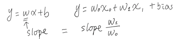
Training accuracy helps monitor how it goes through training, the weights are the parameters neuron learned from given data, i.e. the training set. Let’s try to dive into what exactly does these 3 weights mean.
Through the given instance, we wrote an object function in advance, to see if the neuron could perform its job well: “ line fitting “.
The equation is : y = 5*x -2.
Let’s try to composite above weights:
weight_0x + weight_1y +weight_2*bias = 0
-0.278x + 0.054y + 0.113 = 0 (bias is 1 here)
54y = 278x - 113
y = 5.148x - 2.09
Very close to the object function.
To recap, the goal is to learn a fitting function, which close the object or target function.
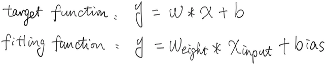
After learning process is done, the outcomes are the weights according to feeded training data. In a linear classification case, we may found the 2 functions share similar slope.
To be continued in Grade 3:
Increase network complexity, let’s see what amazing job could the network perform by just adding 1 more neuron to the network.
[post status: almost done]