Neural Network [grade 3]

Neural Network XOR problem

grade 3: double perceptron with xor problem

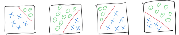
In previous challenge, neural network grade 2, we have managed to make a linear classifier, which as denoted in the following image, could split 2 classes in 2D space.

While, in real world challenge, single linear classifier is not powerful enough, to help us solve transformation like following:

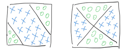
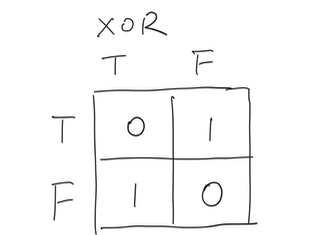
In such scenarios, a single line could not perform the classification tasks well. In computing language, the above scenarios is: XOR.

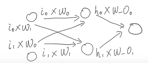
To solve the XOR problem, our network will make a small step, from one single neuron as below:

Upgrade to 2 neuron, as denoted in “blue” as following.

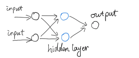
We call the layer in blue as hidden layer, the network now has 3 layers of: input, hidden and output layers. Although the network structure is changed, the feed forward processing is likely remained unchanged in philosophy: transform information forward.

Each node from each layer talks to each node from neighbor layer.

With regards to the training process, we will introduce a new terminology: back propagation.

In previous post, with simple single perceptron neural network grade 2, we measure error as:

    Error = Actual - Predict
    weights += learning_rate * error * inputs

With multi hidden layer network, the formula is kept similar:

    delta_weight = learning_rate * error * gradient(1) * inputs(2)

(1): Purpose for introducing gradient, is to find an effective slope of optimization.

And we have a convenient way for calculating the gradient:

\[s'(x)= s(x) * (1-s(x))\]

Following is the implementation about calculate derivate of sigmoid:

\[s(x) = sigmoid(x) = \frac{1}{1+e^{-x}}\] \[let \: t = 1 + e^{-x}\] \[\frac{d(s)}{d(t)} = -t^{-2}\] \[\frac{d(t)}{d(x)} = -e^{-x}\] \[\frac{d(s)}{d(x)} = -t^{-2} * -e^{-x} = \frac{e^{-x}}{t^2}=\frac{e^{-x}}{(1+e^{-x})^2}\] \[1 - s(x) = \frac{e^{-x}}{1+e^{-x}}\] \[s(x) = \frac{1}{1+e^{-x}}\] \[s'(x)= \frac{e^{-x}}{(1+e^{-x})^2} = s(x) * (1-s(x))\]

As we can see it’s easy to calculate the derivate, so we use sigmoid as activation function has the computational reason. Now let’s have an implementation of back propagation process:

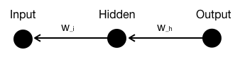
Assume we have a simplified network, which consists of : 1 node for input layer, denotes as “I”, 1 node for hidden layer, denote as “H”, and one node for output layer denote as “O”.

Say target output is “1” or “0”, denote as “Y”, we then have the error or cost as:

\[Error = (O_{utput-activated} - Y)^2\] \[O_{utput-activated} = \sigma (H_idden * W_h + Bias)\] \[\sigma = \frac{1}{1 + e^{-x}}\] \[O_{utput} = H_idden * W_{hidden} + Bias\]

Here we use sigmoid as activate function. The purpose for us doing back propagation is to measure how much impact does the “weight” contribute to the output, by tuning the weight, we make the output moves towards “expect” direction.

Following is how we measure the impact of “W_h” to the output:

\[\frac{\partial Error}{\partial W_h} = \frac{\partial Error}{\partial O_{utput-activated}} * \frac{\partial O_{utput-activated}}{\partial O_{utput}} * \frac{\partial O_{utput}}{\partial W_{hidden}}\]

This is what we called “chain rule”. Now let’s figure out how to implement the chain rule:

\[\frac{\partial Error}{\partial O_{utput-activated}} = 2(O_{utput−activated} −Y)\] \[\frac{\partial O_{utput-activated}}{\partial O_{utput}} = \sigma'\] \[\sigma'(x)= \sigma(x) * (1-\sigma(x))\] \[\frac{\partial O_{utput}}{\partial W_{hidden}} = Hidden\]

Now bring back learning rate and ignore the constant number 2, the fomula turns into:

\[\frac{\partial Error}{\partial W_{hidden}} = learningrate * (O_{utput−activated} −Y) * \sigma(x) * (1-\sigma(x)) * Hidden\]

Calculate “W_i” to the output:

\[\frac{\partial Error}{\partial W_i} = \frac{\partial Error}{\partial H_{idden-activated}} * \frac{\partial H_{idden-activated}}{\partial H_{idden}} * \frac{\partial H_{idden}}{\partial W_{input}}\] \[\frac{\partial Error}{\partial H_{idden-activated}} = 2(O_{utput−activated} −Y) * W_{hidden}\] \[\frac{\partial H_{idden-activated}}{\partial H_{idden}} = \sigma'\] \[\sigma'(x)= \sigma(x) * (1-\sigma(x))\] \[\frac{\partial H_{idden}}{\partial W_{input}} = Input\]

Now bring back learning rate and ignore the constant number 2, the fomula turns into:

\[\frac{\partial Error}{\partial W_{input}} = learningrate * Error * W_{hidden} * \sigma(x) * (1-\sigma(x)) * Input\]

A very good intuitive online tutorial about back propagation is cs231n by Andrej Karpathy.

We have done the implementation of back propagation. Expand to multi-nodes in multi-layers, the methodology applies in the same way, we just sum up the correspond errors and previous layers’ values.

The process of back propagation is the way to figure out derivatives, and we should bear in mind, though deep neural network could be a very heavy in computation, as in graph computing, the powerful derivative tool helped us save a lot and make it achievable in deep neural network computation.

(2): The inputs here could be referred to output layer or hidden layer as multi layer network was imported here. The matrix of output layer / hidden layer should be transposed in implementation, which will be introduced later.

    // Generate the Hidden Outputs
    Matrix inputs = fromArray(input_array);
    Matrix hidden = multiply(weights_ih, inputs);
    hidden.add_m(bias_h);
    hidden = sigmoidMatrix(hidden);
    
    // Generate output layer
    Matrix outputs = multiply(weights_ho, hidden);
    outputs.add_m(bias_o);
    outputs = sigmoidMatrix(outputs);

    // Convert array to matrix object
    Matrix targets = fromArray(target_array);

    // error = targets - outputs
    Matrix output_errors = subtract(targets, outputs);

    // gradient = outputs * (1 - outputs);
    Matrix gradients = dsigmoidMatrix(outputs);
    gradients.multiply_m(output_errors);
    gradients.multiply_n(learning_rate);

    // calculate deltas
    Matrix hidden_T = transpose(hidden);
    Matrix weights_ho_deltas = multiply(gradients, hidden_T);

    // adjust the weights by deltas
    weights_ho.add_m(weights_ho_deltas);
    // adjust the bias by its deltas (which is just the gradients)
    bias_o.add_m(gradients);

    // calculate the hidden layer errors
    Matrix who_t = transpose(weights_ho);
    Matrix hidden_errors = multiply(who_t, output_errors);

    // calculate the hidden gradient
    Matrix hidden_gradient = dsigmoidMatrix(hidden);
    hidden_gradient.multiply_m(hidden_errors);
    hidden_gradient.multiply_n(learning_rate);

    // calculate input->hidden deltas
    Matrix inputs_T = transpose(inputs);
    Matrix weights_ih_deltas = multiply(hidden_gradient, inputs_T);

    weights_ih.add_m(weights_ih_deltas);
    // adjust the bias by its deltas (which is just the gradients)
    bias_h.add_m(hidden_gradient);

[Complete codes on github] https://github.com/hifreedo/nnfs

The above animation is the output of the code hosted in github, each block denotes an input array, and closer to 1 of the output, the darker will it looks like. The animation denotes starts from gray, and after 5000 runs training, which solved the XOR issue successfully.

An intuitive understanding about “2 hidden nodes network structure” will bring significant impact is, if one hidden node denotes a single split line, 2 denotes 2 lines, 3 denotes 3 lines and more …

Put this scenario in a real world, with bricks, arbitrary curve of shape could be paved. Put back into the mathematical world, with multi-layers neural network been introduced, it can perform “curve fitting” job well :)

Yes, deep neural network is about “curve fitting”.

[post status: almost done]

---

Appendix:

Following is the source code of Caffe, which implements sigmoid in forward and backward computing:

namespace caffe {

template <typename Dtype>
inline Dtype sigmoid(Dtype x) {
  return 0.5 * tanh(0.5 * x) + 0.5;
}

template <typename Dtype>
void SigmoidLayer<Dtype>::Forward_cpu(const vector<Blob<Dtype>*>& bottom,
    const vector<Blob<Dtype>*>& top) {
  const Dtype* bottom_data = bottom[0]->cpu_data();
  Dtype* top_data = top[0]->mutable_cpu_data();
  const int count = bottom[0]->count();
  for (int i = 0; i < count; ++i) {
    top_data[i] = sigmoid(bottom_data[i]);
  }
}

template <typename Dtype>
void SigmoidLayer<Dtype>::Backward_cpu(const vector<Blob<Dtype>*>& top,
    const vector<bool>& propagate_down,
    const vector<Blob<Dtype>*>& bottom) {
  if (propagate_down[0]) {
    const Dtype* top_data = top[0]->cpu_data();
    const Dtype* top_diff = top[0]->cpu_diff();
    Dtype* bottom_diff = bottom[0]->mutable_cpu_diff();
    const int count = bottom[0]->count();
    for (int i = 0; i < count; ++i) {
      const Dtype sigmoid_x = top_data[i];
      bottom_diff[i] = top_diff[i] * sigmoid_x * (1. - sigmoid_x);
    }
  }
}