PCA and related
PCA and related
Principal component analysis is a methodology widely implemented in dimensionality reduction.
PCA relies on orthogonal transformation, to covert a set of possibly correlated variables into a set of linearly independent / uncorrelated variables, which were called principal components.
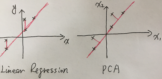
PCA & Linear Regression
The difference between PCA & linear regression, to the latter, the cost function is:
\[argmin\frac{1}{2}(h(\Theta)-y)^2\]While the measurement for PCA is different. The optimization is to lead to:
- maximum variance (which remains maximum original data information)
- minimum covariance (which eliminates correlated dimensions)
In my personal view, the cost function & optimization methodology may be swap between these two, it’s mainly due to established by usage and for the sake of easy to implementation.
First of all, we make zero mean of all the data.
\[Var(a) = \frac{1}{n}\sum_{i=1}^{n}(a - \bar{a})^2\] \[Cov(a, b) = \frac{1}{n}\sum_{i=1}^{n}(a - \bar{a})(b-\bar{b}) = \frac{1}{n}\sum_{i=1}^{n}ab\]Our initiative is to maximize Var(a) and minimize Cov(a,b).
And there’s a perfect equation on this:
\[\frac{1}{n}XX^T\]According to definition of covariance matrix, which consists of variance of variables along the main diagonal and the covariance between each variables in the other matrix positions.
So, the leads is clear now: Try to maximize the values along the main diagonal and sort them by descend, and minimize the other values through the matrix.
Though tends to minimize information loss, it’s a “lossy compression”.
Steps of calculating PCA
- Zero mean of dataset;
- Covariance matrix;
- Eigenvectors & eigenvalues;
- Decide top K values;
A practice for deciding K:
\[\frac{\sum_{i=0}^{k}\lambda_k}{\sum_{i=0}^{n}\lambda_n} \geqslant 0.99\]PCA & SVD
| PCA | SVD | |
|---|---|---|
| purpose | dimensionality reduction | matrix decomposition |
| sparse data | not support, zero mean data | supports sparse matrix |
| computation | less efficient, needs solve cov matrix | efficient |
| reduction | one way, dimensionality | bilateral, dimensionality(right matrix) and sample numbers(left matrix) |
Towards bilateral dimensionality reduction, let’s assume we have input data set m*n. According to SVD:
\[SVD = U_{m,r}\sum_{r,r}V_{r,n}^T\] \[New = U_{m,r}^TX_{m,n}\]By transformation, we may get a new matrix with r * n, here we managed to reduct the rows from the original data set, that’s another way of data set reduction.
PCA is more than dimensionality reduction
Other than dimensionality reduction, PCA was introduced into image argumentation with the “ImageNet Classification with Deep Convolutional Neural Network” aka AlexNet.
According to the paper, Alex et.al decreased top 1 error rate by 1% in imagenet, which was pretty amazing.
The method is:
\[NewImage = [p_1, p_2, p_3][\alpha_1\lambda_1,\alpha_2\lambda_2,\alpha_3\lambda_3 ]\]Where p is the eigen vector, lambda is eigen value, alpha is Gaussian random with zero mean and std variation 0.1.
[post status: half done]