Neural Network [grade 5]
Neural Network solving mnist
grade 5: Mini version of mnist classification
The mnist solving is a big milestone for neural network practice in real field.
We will present a workable mini version, in this version, the main items and challenges will be went through.
To get started, you will need to download mnist dataset in csv format, the dataset is pretty easy to be found online. There are 2 csv files: 1 for training, 60k images in toal, and 1 for test, 10k images. Each line represents an image, 785 columns in total, 1st number denotes a label (from 0 to 9), the following 784 numbers denote the 28*28 pixels image.
The core part: “train function” in neural network as following, is no more than 20 lines of code. Yet with these 20 lines, in 30 epochs, the model could achieve up to 97.76% accuracy in training set, which means among 10,000 images, only 240 images was misclassified.
This is quite amazing result, the back propagation algorithm is easy to understand and not difficult to implement, yet could achieve better classification result than the other algorithms, such as: SVM, KNN, Random Forest etc.
To achieve above performance of 97.6% in the mini 2 layers’ network (1 hidden layer and 1 output layer, we do not count the input layer in, because it won’t participate in the calculation), you will need to pay attention to the following key points, otherwise you won’t be able to reproduce, or even could not make the network work in a reasonable way.
Key points:
- Feature scaling , scale the training data from (0 to 255) to (0 to 1). Take the simple min max normalization, is to divide by 255 to each number.
- Weights distribution, to make sure the random assigned weights to the input nodes and hidden nodes, are aligned with standard normal distribution, they should have positives and negatives, instead of common mistakes: all positive or all in 0 to 1.
- Reasonable network structure and hyper parameters: the input and output nodes are fixed numbers, 784 and 10. The hidden layer nodes are suggested to take a number between 100 to 400, it’s a balance need to make between efficiency and accuracy. You might make a network with 1000 hidden nodes work and yield good performance, but which will take way longer time to train. As the learning rate, suggestion is to tune around 0.1.
Alright now, before dive into constructing the network by hand, take a deep breath, go through feed forward and back propagation on the paper, look out and there are traps need to pay attention to:
- The bias, with adding bias, the dimension of inputs & hidden layer will by changed. Hence the weights’ dimensions will be changed accordingly.
- The matrix transformation, need to be conducted in both feed forward and back propagation process.
In a network structure with bias of : 784 input nodes, 100 hidden nodes, 10 output nodes, the forward and backward processing looks as following:
inputs = inputs + bias = [ 1 * 785]
inputs.transform = [785 * 1]
labels.transform = [10 * 1]

hidden_layer = wih (100 * 785) dot inputs (785 *1) = [100 * 1]
hidden_layer->activate

hidden_layer = hidden_layer + bias = [101 * 1]
out_layer = who (10 * 101) dot hidden_layer (101 * 1) = [10 * 1]
out_layer->activate

out_errors = labels(10 * 1) - out_layer(10 * 1) = [10 * 1]
gradients = out_errors(10 * 1) * dactivate(out_layer) (10 * 1)
gradients = learning_rate * gradients = [10 * 1]
who_delta = gradients(10 * 1) dot hidden_layer.transform(1 * 100) = [10 * 101]
who = who_delta(10 * 101) + who(10 * 101) = [10 * 101]

hidden_errors = who.transform (101 * 10) dot out_errors(10 * 1) = [101 * 1]
gradients = hidden_layer->deactivate
gradients = hidden_errors (101 * 1) * gradients (101 * 1) = [101 * 1]
gradients = learning_rate * gradients = [101 * 1]
wih_delta = gradients (101 * 1) dot inputs.transform (1 * 785) = [101 * 785]
wih_delta = wih_delta[:-1, :] = [100 * 785]
wih = wih_delta (100 * 785) + wih (100 * 785) = [100 * 785]
Code implementation with python 3 in notebook:
# mnist mini version
from __future__ import print_function, division
import numpy as np
import matplotlib.pyplot as plt

# prepare training
img_size = 28
img_pixel = 28*28
num_label = 10

# read data, needs to be downloaded in advance
train_set = np.loadtxt("dataset/mnist/mnist_train.csv", delimiter=",")
test_set = np.loadtxt("dataset/mnist/mnist_test.csv", delimiter=",")

# get test, train sets and labels
train_label, train_img = np.asfarray(train_set[:, :1]), np.asfarray(train_set[:, 1:]) / 255
test_label, test_img = np.asfarray(test_set[:, :1]), np.asfarray(test_set[:, 1:]) / 255

# make one hot labels
one = np.arange(num_label)
train_label_onehot = (one == train_label).astype(np.float)
test_label_onehot = (one == test_label).astype(np.float)

# review data
for i in range(10):
    data = train_img[i].reshape(28, 28)
    plt.imshow(data)
    plt.show()
# activation function & derivative
def sigmoid(x):
    return 1 / (1 + np.exp(-x))

def dsigmoid(x):
    return x * (1 - x)

class NeuralNetwork():
    def __init__(self, _num_in_nodes, _num_hidden_nodes, _num_out_nodes, _lr, _activate, _dactivate, _bias=1):
        self.num_in_nodes = _num_in_nodes
        self.num_hidden_nodes = _num_hidden_nodes
        self.num_out_nodes = _num_out_nodes
        self.lr = _lr
        self.activate = _activate
        self.dactivate = _dactivate
        self.bias = _bias

        # init weights, +1 is the bias node
        self.wih = np.random.randn(self.num_hidden_nodes, self.num_in_nodes + 1)
        self.who = np.random.randn(self.num_out_nodes, self.num_hidden_nodes + 1)

    def train(self, inputs, labels):
        # calcuate output and errors
        inputs = np.concatenate((inputs, [self.bias]))
        inputs = np.array(inputs, ndmin=2).T
        labels = np.array(labels, ndmin=2).T

        hidden_layer = np.dot(self.wih, inputs)
        hidden_layer = self.activate(hidden_layer)

        hidden_layer = np.concatenate((hidden_layer, [[self.bias]]))
        output_layer = np.dot(self.who, hidden_layer)
        output_layer = self.activate(output_layer)

        output_errors = labels - output_layer

        # start backpropagation for who
        gradients = output_errors * self.dactivate(output_layer)
        gradients = self.lr * gradients
        who_delta = np.dot(gradients, hidden_layer.T)

        self.who += who_delta

        # backpropagation for wih
        hidden_errors = np.dot(self.who.T, output_errors)
        gradients = self.dactivate(hidden_layer)
        gradients = hidden_errors * gradients
        gradients = self.lr * gradients
        wih_delta = np.dot(gradients, inputs.T)[:-1, :]

        self.wih += wih_delta

    def run(self, inputs, labels, epochs=1):
        # multiple runs
        for epoch in range(epochs):
            for i in range(len(inputs)):
                self.train(inputs[i], labels[i])

    def predict(self, inputs):
        # generate output based inputs
        inputs = np.concatenate((inputs, [self.bias]))
        inputs = np.array(inputs, ndmin=2).T
        hidden_layer = np.dot(self.wih, inputs)
        hidden_layer = self.activate(hidden_layer)

        hidden_layer = np.concatenate((hidden_layer, [[self.bias]]))
        output_layer = np.dot(self.who, hidden_layer)
        output_layer = self.activate(output_layer)

        return output_layer

    def evaluate(self, inputs, labels):
        # evaluate result
        correct, wrong = 0, 0
        for i in range(len(inputs)):
            res = self.predict(inputs[i])
            res_max = res.argmax()
            if res_max == labels[i]:
                correct += 1
            else:
                wrong += 1
        return correct, wrong

_activate = sigmoid
_dactivate = dsigmoid
_num_in_nodes = 784
_num_hidden_nodes = 100
_num_out_nodes = 10
_lr = 0.1
_bias = 1
NN = NeuralNetwork(_num_in_nodes, _num_hidden_nodes, _num_out_nodes, _lr, _activate, _dactivate, _bias)

epochs = 2
for i in range(epochs):
    NN.run(train_img, train_label_onehot, 1)
    correct, wrong = NN.evaluate(train_img, train_label)
    print("epoch {0}".format(i))
    print("train precision: {0}".format(correct / (correct + wrong)))
    correct, wrong = NN.evaluate(test_img, test_label)
    print("test precision: {0}".format(correct / (correct + wrong)))
Following is an experiment, with parameters as:
- Input nodes: 784
- Hidden nodes: 100
- Output nodes: 10
- Learning_rate: 0.1
- Bias: 1
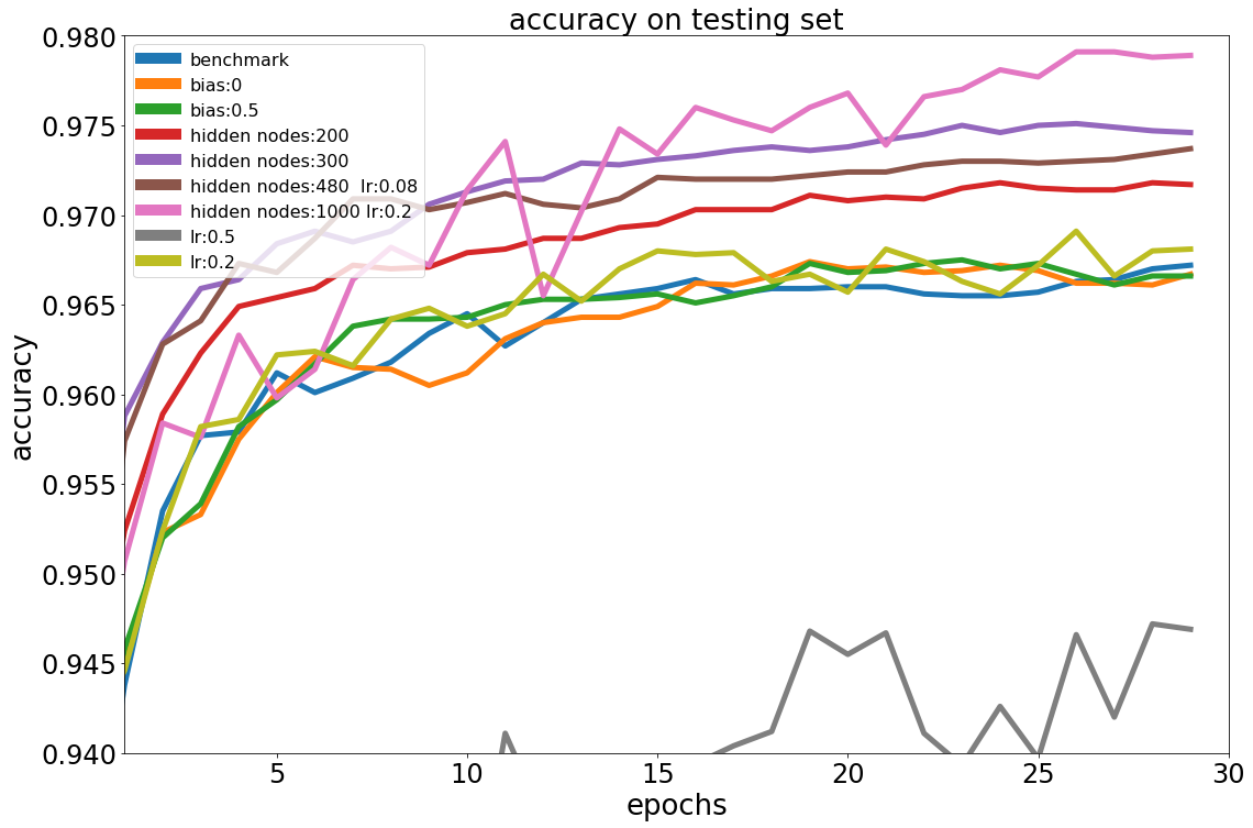
Use the above settings as benchmark, then wiggle the parameters from different perspective. For each experiment, will run 30 epochs.
A few observations through the experiments:
-
Set bias to 0, 0.5, 1 doesn’t make observable difference.Greater than 0.1 on learning rate side doesn’t make good on performance either.
-
Performance goes up while increasing number of hidden nodes (up to 97.79%), especially when set the number to 1000, on the other hand, the training time increases significantly, take 10X times compares to the benchmark with 100 hidden nodes.
So, we may consider to have a solid network structure first, then tune the hyper parameters.
When we dealing with a fixed depth neural network, it seems better performance still could be achieved by increasing width of network, even have number of nodes from middle layer bigger than number of input nodes, for e.g. set the hidden layer nodes 1000 compares to inputs of 784. And of course, the training time is dramatically increased.
Towards current network structure: a large net (from width perspective, slightly bigger than input nodes) might give you some good, only if you could bare with training cost. A large learning rate, greater than 1, definitely could not supply any of goods on both performance and efficiency.
There’s also another experiment conducted to test the way of learning rate choosing:
lr_upper_bound = 0.18  # according to exp observation
lr_lower_bound = 0.04  # same as above

# get lr by random
lr_set_random = np.random(lr_upper_bound, lr_lower_bound, 30)

# get lr by interval
interval = (lr_upper_bound - lr_down_bound) / 30
lr_set_interval = [(0.04 + interval * i) for i in range(30)]
We choose learning rate randomly in a given range and for each learning rate, run 22 epochs and get the best performance in test set.
The other way is, choose learning rate by interval equally, run same epochs and get best result. Following is the result of these 2 groups:
lr_random_performance = [0.9692, 0.9659, 0.9698, 0.9655, 0.9695, 0.9691, 0.9647, 0.966, 0.9675, 0.9681, 0.9665, 0.9643, 0.9651, 0.9677, 0.9675, 0.9662, 0.97, 0.9669, 0.969, 0.9704, 0.9679, 0.9682, 0.9641, 0.9658, 0.9685, 0.9676, 0.9644, 0.9673, 0.9685]
lr_interval_performance = [0.9644, 0.9639, 0.9642, 0.9657, 0.9636, 0.9678, 0.9695, 0.9684, 0.9655, 0.9681, 0.9677, 0.9657, 0.9653, 0.9676, 0.9674, 0.9681, 0.9708, 0.9713, 0.9682, 0.967, 0.9704, 0.9716, 0.9683, 0.9686, 0.969, 0.9691, 0.9677, 0.9684, 0.9705]
To check if these 2 methodologies under “current circumstance” has statistical significance, we make null hypothesis as there are no difference.
We will run students’ t-test to validate the null hypothesis:
from scipy import stats

# run variances check see if equal
stats.levene(group1, group2)
# LeveneResult(statistic=0.31839523311861617, pvalue=0.574826791825623)

# run normality test
stats.shapiro(group1)
stats.shapiro(group2)
# (0.9579369425773621, 0.2921314537525177)

# both groups follow normal distribution and share same variance, now we could run t-test
stats.ttest_ind(max_tmp, max_tmp2, equal_var = True)
# Ttest_indResult(statistic=-0.8177164769659798, pvalue=0.41698479611664985)
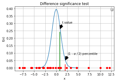
Under current experiment circumstance and significance level of 0.05, the null hypothesis was accepted, there’s no difference between choose random or interval learning rate.
And you might also take this into consideration, what will the accuracy be after run many epochs if we set the learning rate as negative value?
As said, this is the mini version of mnist classification, in the coming future posts, various activation functions, multi hidden layers, L1 and L2 normalization and batch normalization methods will be introduced into coming versions.
[post status: almost done]