Convolution in forward and backward

Convolution in forward and backward

Convolution neural network is a specific type of MLP, multi-layer perceptron, yet it complies with MLP’s core, which is: \(y = w*x + b\)

With x been transferred forward, to get a cost function (which is a scalar) of:

\(J(\theta, x, y)\) We then back propagate the J function, with gradient descent methodology, to compute: \(\frac{\partial J(\theta, x, y)}{\partial \theta}\)

Once done optimization with cost function J, which means we could get the representation parameters with given training data x and label data y.

Following is a simplified convolution network, let’s assume an image input with 1 channel, a kernel filter with 1 channel and an output with padding on input layer, which makes the output size is same as input.

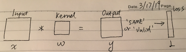
We have: $\frac{\partial L}{\partial y}$ already known.

2 unknowns going to be solved:

\[\frac{\partial L}{\partial w} \qquad and \qquad \frac{\partial L}{\partial x}\]

Part 1:

According to “chain rule” in calculus,

\[\frac{\partial L}{\partial w} = \frac{\partial L}{\partial y} * \frac{\partial y}{\partial w}\] \[\frac{\partial L}{\partial w} = \frac{\partial L}{\partial y} * \frac{\partial {(x * w)}}{\partial w} = \frac{\partial L}{\partial y} * x^T\]

How does this magic $x^T$ comes out?

Well, let’s review the traditional & im2col convolutional process again, you may easily find more reference infos about traditional & im2cold through web.

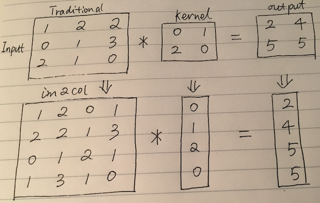
Here we’d like to emphasize that, through the im2col method, we may transfer convolutional to matrix product.

And if we simplify kernel into just one kernel, this actually turns into “jacobian matrix”, by doing that, the kernel and output both turns into “column vector”.

Following is an explanation intuitively about why there is an $x^T$.

\[x = \begin{bmatrix} x_1, x_2, x_3 \end{bmatrix} \quad w = \begin{bmatrix} w_1 \\ w_2 \\ w_3 \end{bmatrix} \\ y = xw = x_1w_1 + x_2w_2 + x_3w_3 \\ \frac{\partial y}{\partial w} = \begin{bmatrix} \frac{\partial y}{\partial w_1} \\ \frac{\partial y}{\partial w_2} \\ \frac{\partial y}{\partial w_3} \end{bmatrix} = \begin{bmatrix} x_1 \\ x_2 \\ x_3 \end{bmatrix} = x^T\]

Part 2:

According to “chain rule” in calculus,

\[\frac{\partial L}{\partial x} = \frac{\partial L}{\partial y} * \frac{\partial y}{\partial x}\]

We have $\frac{\partial L}{\partial y}$ already known, and going to figure out $\frac{\partial y}{\partial x}$.

With saying $\frac{\partial y}{\partial x}$, the factor behind the scene is, what’s the scope of impact with one unit chaning on “x” will put on “y”.

Let’s take a look at the convolution procedure again:

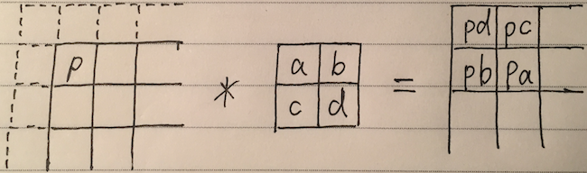
Take a pixel from upper left of the input, say “p”. What’s the scope of impact of “p”, will put on output “y”?

Through the 22 kernel, we could see 1 pixel from “x” will affect 22 pixels in “y”, in the sequence of “pd, pc, pb, pa”.

A little bit details on how do we get the “pd, pc, pb, pa”:

With 22 kernel and stride 1, we could find out the output value of y on the upper left equals to: pd + f(rest3pixels * rest3weights), in short p*d + f(c) .

2 notices: in order keep output size is equal to the input x, we added padding in x, denoted by line of dashes. The f(c) is not important, because when calculating derivative of $\frac{\partial y_p}{\partial x_p}$ , the f(c) will be eliminated.

Now let’s move back to the implementation, we have:

\[p * kernel(a, b , c , d) = {pd, pc, pb, pa}\]

This is exactly:

\[p * kernel^{flip} = {pd, pc, pb, pa}\]

What an interesting finding!

By solving $\frac{\partial y_p}{\partial x_p}$, we now get:

\[\frac{\partial L}{\partial x} = \frac{\partial L}{\partial y} * w^{flip}\]

Let’s find out more about the multiplication:

Assume size of input is: $N_1 * N_2$ and size of kernel is $K_1 * K_2$, we know size of output is the same as input: $N_1 * N_2$

\[|\frac{\partial L}{\partial y}| = N_1 * N_2 \qquad |w^{flip}| = K_1 * K_2\]

Hence, this is another convolution.

To recap, on calculating $\frac{\partial L}{\partial w}$, we transfer the convolution into the matrix multiplication by im2col method.

On calculating $\frac{\partial L}{\partial x}$, we take out 1 pixel from input to observe the consequence in the output.

With this in mind, let’s come to the conclusion:

Conclusion:

The forward process is convolution.

The backward process is also convolution, with flipped kernel.

[post status: almost done]