Neural Network [grade 4]
Neural Network with L1 and L2
grade 4: regularization L1 and L2
The intuition about L1 and L2 in neural network, is about to train the net with efficiency and avoid of over fitting.
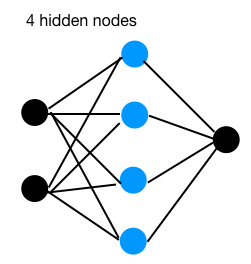
Following are 3 nets with different number of hidden nodes:
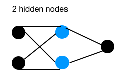
A brief view of above 3 nets:
With the 3 different networks, we perform an xor problem, the target is to get 99% accuracy on training set. Once hits the target, record the weights of the 3rd layer as following:
| hidden nodes | weights |
|---|---|
| 2 | 9.7 9.6 |
| 4 | -3.4 -4.5 -4.7 4.9 |
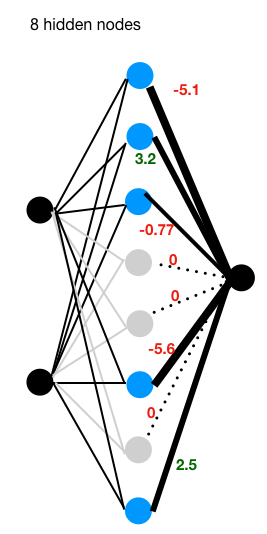
| 8 | -0.13 -0.58 -1.3 -1.3 -3.2 0.95 2.7 3.6 |
As we tested in previous post: neural network for xor problem, a network consists of 2 hidden nodes could just do the classification job, though with a little inefficient, you may got 1 shot on 10 trials. As we know, with only 2 nodes, in case one node represents the weight in wrong direction, it’s quite hard for the network to correct to the right direction.
With hidden nodes of 4, the network seems could perform the xor problems well, for each time it could converge to the target accuracy, end with somehow equal weights (with absolute value), which means, all of the 4 nodes plays important representative roles.
When comes to hidden nodes of 8, compares with structures of hidden nodes of 4, there are 3 nodes (with absolute weight) close to zero. Which means, these 3 nodes are somehow redundant.
With the network goes wider (more hidden nodes on single layer) and deeper (more layers), it has stronger power of representation. Things come with pros and cons, with “bigger” network there are higher risk on over fitting and consumes more computation source.
With introduction of L1 and L2, which aims to minimize over fitting by squeeze some “outlier” weights close or equals to zero. Take a look at the 3rd image of “8 hidden nodes”, under L1 regularization terms, there are 3 nodes’(in color gray) weight been set to zero, which means they are inactive in the network and will not join further feed and back propagation. With the rest of 5 nodes, the network performs the xor job well.
The L1 puts similar effect like “drop out” in 3rd image, we will not introduce all of the methodologies of avoiding over fitting in this post.
L1 regularization:
\[W = MSE + \lambda\sum_{i=1}^k|w_i|\]L2 regularization:
\[W = MSE + \lambda\sum_{i=1}^kw_i^2\]| Comparison | L1 regularization | L2 regularization |
|---|---|---|
| Computation | Inefficient on non-sparse | Efficient |
| Outputs | Sparse | Non-sparse |
| Feature selection | Yes, some set to 0 | No selection |
Following is an image borrowed from wikipedia:
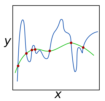
To explain intuition from another way, on the image, green line function could generalize better to underlying unknown distribution points, the blue line seems yield too much to each individual points that leads to over fitting. (Actually I may change the image to another better one letter).
Let’s say the green one equals to :
\[y = 2 + 3x + 4x^2\]and the blue one, a higher-degree polynomial function :
\[y = 2 + 3x + 4x^2 + 5x^3 + 6x^4 + 7x^5\]We want to eliminate 5 , 6, 7. In practice, we don’t know which one to eliminate, what we do is add up them all, and apply the squeeze to all of them.
On doing the “squeeze” processing, for L1 some features / weights will be set to zero, we may think in a way that L1 is the process of subtract a small part for each time, and for L2, some weights will be set to very close to zero but will not be zero, we may think L2 is to multiply a small proportion each time.
The $\lambda$ here is the hyper-parameter, if set to zero, then means there will be no regularization, if set to infinite, what we will get is likely all of the weights been set to zero. Like the function (4), which will be turned into:
\[y = 2\]It’s a flat line, which means the model goes to another extreme direction: no capability of representative, aka under fitting.
Though this post, we are pushing the neural network model in a way of complexity: properly choose hidden nodes, regularization and hyper-parameter $\lambda$.
[post status: half done]